
Author’s note: July 13th 9:02am PT – Corrected number of test files and related calculations.
A browser is an incredibly complex piece of software. With such enormous complexity, the only way to maintain a rapid pace of development is through an extensive CI system that can give developers confidence that their changes won’t introduce bugs. Given the scale of our CI, we’re always looking for ways to reduce load while maintaining a high standard of product quality. We wondered if we could use machine learning to reach a higher degree of efficiency.
Continuous integration at scale
At Mozilla we have around 85,000 unique test files. Each contain many test functions. These tests need to run on all our supported platforms (Windows, Mac, Linux, Android) against a variety of build configurations (PGO, debug, ASan, etc.), with a range of runtime parameters (site isolation, WebRender, multi-process, etc.).
While we don’t test against every possible combination of the above, there are still over 90 unique configurations that we do test against. In other words, for each change that developers push to the repository, we could potentially run all 85k tests 90 different times. On an average work day we see nearly 300 pushes (including our testing branch). If we simply ran every test on every configuration on every push, we’d run approximately 2.3 billion test files per day! While we do throw money at this problem to some extent, as an independent non-profit organization, our budget is finite.
So how do we keep our CI load manageable? First, we recognize that some of those ninety unique configurations are more important than others. Many of the less important ones only run a small subset of the tests, or only run on a handful of pushes per day, or both. Second, in the case of our testing branch, we rely on our developers to specify which configurations and tests are most relevant to their changes. Third, we use an integration branch.
Basically, when a patch is pushed to the integration branch, we only run a small subset of tests against it. We then periodically run everything and employ code sheriffs to figure out if we missed any regressions. If so, they back out the offending patch. The integration branch is periodically merged to the main branch once everything looks good.
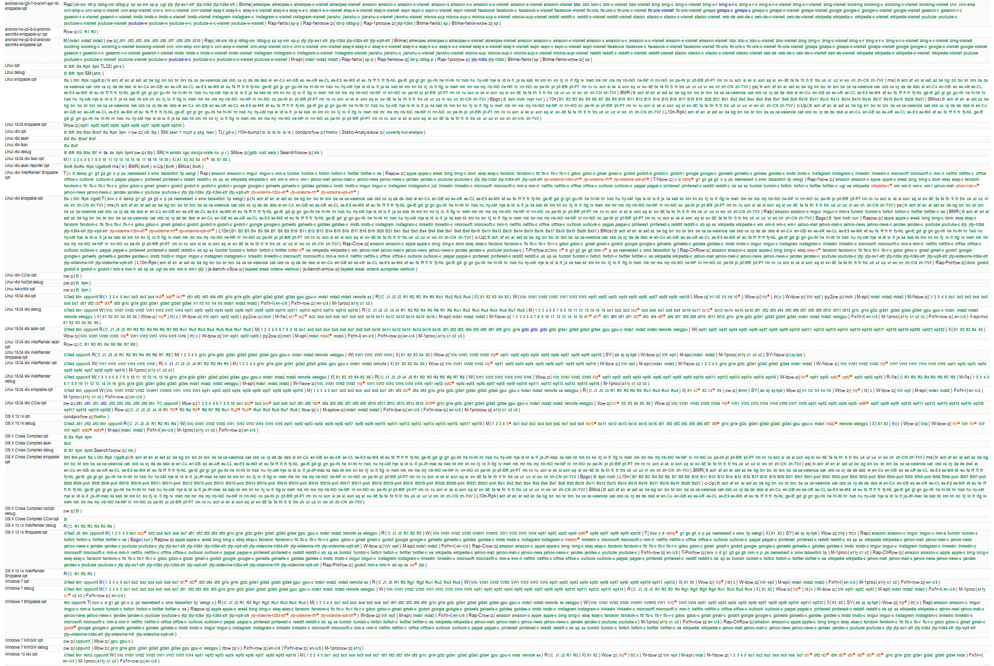 A subset of the tasks we run on a single mozilla-central push. The full set of tasks was too hard to distinguish when scaled to fit in a single image.
A new approach to efficient testing
These methods have served us well for many years, but it turns out they’re still very expensive. Even with all of these optimizations our CI still runs around 10 compute years per day! Part of the problem is that we have been using a naive heuristic to choose which tasks to run on the integration branch. The heuristic ranks tasks based on how frequently they have failed in the past. The ranking is unrelated to the contents of the patch. So a push that modifies a README file would run the same tasks as a push that turns on site isolation. Additionally, the responsibility for determining which tests and configurations to run on the testing branch has shifted over to the developers themselves. This wastes their valuable time and tends towards over-selection of tests.
About a year ago, we started asking ourselves: how can we do better? We realized that the current implementation of our CI relies heavily on human intervention. What if we could instead correlate patches to tests using historical regression data? Could we use a machine learning algorithm to figure out the optimal set of tests to run? We hypothesized that we could simultaneously save money by running fewer tests, get results faster, and reduce the cognitive burden on developers. In the process, we would build out the infrastructure necessary to keep our CI pipeline running efficiently.
Having fun with historical failures
The main prerequisite to a machine-learning-based solution is collecting a large and precise enough regression dataset. On the surface this appears easy. We already store the status of all test executions in a data warehouse called ActiveData. But in reality, it’s very hard to do for the reasons below.
Since we only run a subset of tests on any given push (and then periodically run all of them), it’s not always obvious when a regression was introduced. Consider the following scenario:
| Test A | Test B | |
| Patch 1 | PASS | PASS |
| Patch 2 | FAIL | NOT RUN |
| Patch 3 | FAIL | FAIL |
It is easy to see that the “Test A” failure was regressed by Patch 2, as that’s where it first started failing. However with the “Test B” failure, we can’t really be sure. Was it caused by Patch 2 or 3? Now imagine there are 8 patches in between the last PASS and the first FAIL. That adds a lot of uncertainty!
Intermittent (aka flaky) failures also make it hard to collect regression data. Sometimes tests can both pass and fail on the same codebase for all sorts of different reasons. It turns out we can’t be sure that Patch 2 regressed “Test A” in the table above after all! That is unless we re-run the failure enough times to be statistically confident. Even worse, the patch itself could have introduced the intermittent failure in the first place. We can’t assume that just because a failure is intermittent that it’s not a regression.
 The writers of this post having a hard time.
Our heuristics
In order to solve these problems, we have built quite a large and complicated set of heuristics to predict which regressions are caused by which patch. For example, if a patch is later backed out, we check the status of the tests on the backout push. If they’re still failing, we can be pretty sure the failures were not due to the patch. Conversely, if they start passing we can be pretty sure that the patch was at fault.
Some failures are classified by humans. This can work to our advantage. Part of the code sheriff’s job is annotating failures (e.g. “intermittent” or “fixed by commit” for failures fixed at some later point). These classifications are a huge help finding regressions in the face of missing or intermittent tests. Unfortunately, due to the sheer number of patches and failures happening continuously, 100% accuracy is not attainable. So we even have heuristics to evaluate the accuracy of the classifications!
 Sheriffs complaining about intermittent failures.
Another trick for handling missing data is to backfill missing tests. We select tests to run on older pushes where they didn’t initially run, for the purpose of finding which push caused a regression. Currently, sheriffs do this manually. However, there are plans to automate it in certain circumstances in the future.
Collecting data about patches
We also need to collect data about the patches themselves, including files modified and the diff. This allows us to correlate with the test failure data. In this way, the machine learning model can determine the set of tests most likely to fail for a given patch.
Collecting data about patches is way easier, as it is totally deterministic. We iterate through all the commits in our Mercurial repository, parsing patches with our rust-parsepatch project and analyzing source code with our rust-code-analysis project.
Designing the training set
Now that we have a dataset of patches and associated tests (both passes and failures), we can build a training set and a validation set to teach our machines how to select tests for us.
90% of the dataset is used as a training set, 10% is used as a validation set. The split must be done carefully. All patches in the validation set must be posterior to those in the training set. If we were to split randomly, we’d leak information from the future into the training set, causing the resulting model to be biased and artificially making its results look better than they actually are.
For example, consider a test which had never failed until last week and has failed a few times since then. If we train the model with a randomly picked training set, we might find ourselves in the situation where a few failures are in the training set and a few in the validation set. The model might be able to correctly predict the failures in the validation set, since it saw some examples in the training set.
In a real-world scenario though, we can’t look into the future. The model can’t know what will happen in the next week, but only what has happened so far. To evaluate properly, we need to pretend we are in the past, and future data (relative to the training set) must be inaccessible.
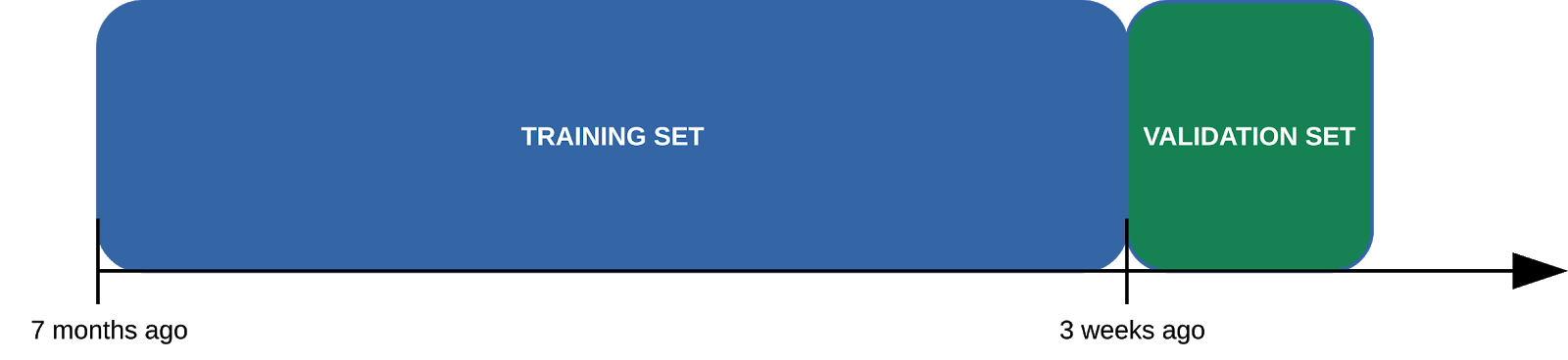 Visualization of our split between training and validation set.
Building the model
We train an XGBoost model, using features from both test, patch, and the links between them, e.g:
- In the past, how often did this test fail when the same files were touched?
- How far in the directory tree are the source files from the test files?
- How often in the VCS history were the source files modified together with the test files?
 Full view of the model training infrastructure.
The input to the model is a tuple (TEST, PATCH), and the label is a binary FAIL or NOT FAIL. This means we have a single model that is able to take care of all tests. This architecture allows us to exploit the commonalities between test selection decisions in an easy way. A normal multi-label model, where each test is a completely separate label, would not be able to extrapolate the information about a given test and apply it to another completely unrelated test.
Given that we have tens of thousands of tests, even if our model was 99.9% accurate (which is pretty accurate, just one error every 1000 evaluations), we’d still be making mistakes for pretty much every patch! Luckily the cost associated with false positives (tests which are selected by the model for a given patch but do not fail) is not as high in our domain, as it would be if say, we were trying to recognize faces for policing purposes. The only price we pay is running some useless tests. At the same time we avoided running hundreds of them, so the net result is a huge savings!
As developers periodically switch what they are working on the dataset we train on evolves. So we currently retrain the model every two weeks.
Optimizing configurations
After we have chosen which tests to run, we can further improve the selection by choosing where the tests should run. In other words, the set of configurations they should run on. We use the dataset we’ve collected to identify redundant configurations for any given test. For instance, is it really worth running a test on both Windows 7 and Windows 10? To identify these redundancies, we use a solution similar to frequent itemset mining:
- Collect failure statistics for groups of tests and configurations
- Calculate the “support” as the number of pushes in which both X and Y failed over the number of pushes in which they both run
- Calculate the “confidence” as the number of pushes in which both X and Y failed over the number of pushes in which they both run and only one of the two failed.
We only select configuration groups where the support is high (low support would mean we don’t have enough proof) and the confidence is high (low confidence would mean we had many cases where the redundancy did not apply).
Once we have the set of tests to run, information on whether their results are configuration-dependent or not, and a set of machines (with their associated cost) on which to run them; we can formulate a mathematical optimization problem which we solve with a mixed-integer programming solver. This way, we can easily change the optimization objective we want to achieve without invasive changes to the optimization algorithm. At the moment, the optimization objective is to select the cheapest configurations on which to run the tests.
| Minimize |  |
| Subject to | 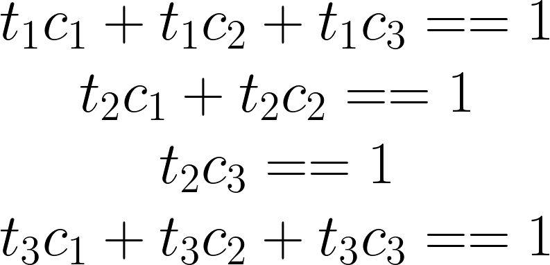 |
| And |  |
Using the model
A machine learning model is only as useful as a consumer’s ability to use it. To that end, we decided to host a service on Heroku using dedicated worker dynos to service requests and Redis Queues to bridge between the backend and frontend. The frontend exposes a simple REST API, so consumers need only specify the push they are interested in (identified by the branch and topmost revision). The backend will automatically determine the files changed and their contents using a clone of mozilla-central.
Depending on the size of the push and the number of pushes in the queue to be analyzed, the service can take several minutes to compute the results. We therefore ensure that we never queue up more than a single job for any given push. We cache results once computed. This allows consumers to kick off a query asynchronously, and periodically poll to see if the results are ready.
We currently use the service when scheduling tasks on our integration branch. It’s also used when developers run the special mach try auto command to test their changes on the testing branch. In the future, we may also use it to determine which tests a developer should run locally.
 Sequence diagram depicting the communication between the various actors in our infrastructure.
Measuring and comparing results
From the outset of this project, we felt it was crucial that we be able to run and compare experiments, measure our success and be confident that the changes to our algorithms were actually an improvement on the status quo. There are effectively two variables that we care about in a scheduling algorithm:
- The amount of resources used (measured in hours or dollars).
- The regression detection rate. That is, the percentage of introduced regressions that were caught directly on the push that caused them. In other words, we didn’t have to rely on a human to backfill the failure to figure out which push was the culprit.
We defined our metric:
scheduler effectiveness = 1000 * regression detection rate / hours per push
The higher this metric, the more effective a scheduling algorithm is. Now that we had our metric, we invented the concept of a “shadow scheduler”. Shadow schedulers are tasks that run on every push, which shadow the actual scheduling algorithm. Only rather than actually scheduling things, they output what they would have scheduled had they been the default. Each shadow scheduler may interpret the data returned by our machine learning service a bit differently. Or they may run additional optimizations on top of what the machine learning model recommends.
Finally we wrote an ETL to query the results of all these shadow schedulers, compute the scheduler effectiveness metric of each, and plot them all in a dashboard. At the moment, there are about a dozen different shadow schedulers that we’re monitoring and fine-tuning to find the best possible outcome. Once we’ve identified a winner, we make it the default algorithm. And then we start the process over again, creating further experiments.
Conclusion
The early results of this project have been very promising. Compared to our previous solution, we’ve reduced the number of test tasks on our integration branch by 70%! Compared to a CI system with no test selection, by almost 99%! We’ve also seen pretty fast adoption of our mach try auto tool, suggesting a usability improvement (since developers no longer need to think about what to select). But there is still a long way to go!
We need to improve the model’s ability to select configurations and default to that. Our regression detection heuristics and the quality of our dataset needs to improve. We have yet to implement usability and stability fixes to mach try auto.
And while we can’t make any promises, we’d love to package the model and service up in a way that is useful to organizations outside of Mozilla. Currently, this effort is part of a larger project that contains other machine learning infrastructure originally created to help manage Mozilla’s Bugzilla instance. Stay tuned!
If you’d like to learn more about this project or Firefox’s CI system in general, feel free to ask on our Matrix channel, #firefox-ci:mozilla.org.
About Andrew Halberstadt
Andrew works on CI, test infrastructure, linting and general developer productivity tooling.
More articles by Andrew Halberstadt…
About Marco Castelluccio
Marco is a passionate Mozilla hackeneer (a strange hybrid between hacker and engineer), who contributed and keeps contributing to Firefox, PluotSorbet, Open Web Apps. More recently he has been working on using machine learning and data mining techniques for software engineering (testing, crash handling, bug management, and so on).
4 comments