The Machine Learning team at Mozilla Research continues to work on an automatic speech recognition engine as part of Project DeepSpeech, which aims to make speech technologies and trained models openly available to developers. We’re hard at work improving performance and ease-of-use for our open source speech-to-text engine. The upcoming 0.2 release will include a much-requested feature: the ability to do speech recognition live, as the audio is being recorded. This blog post describes how we changed the STT engine’s architecture to allow for this, achieving real-time transcription performance. Soon, you’ll be able to transcribe audio at least as fast as it’s coming in.

When applying neural networks to sequential data like audio or text, it’s important to capture patterns that emerge over time. Recurrent neural networks (RNNs) are neural networks that “remember” — they take as input not just the next element in the data, but also a state that evolves over time, and use this state to capture time-dependent patterns. Sometimes, you may want to capture patterns that depend on future data as well. One of the ways to solve this is by using two RNNs, one that goes forward in time and one that goes backward, starting from the last element in the data and going to the first element. You can learn more about RNNs (and about the specific type of RNN used in DeepSpeech) in this article by Chris Olah.

Using a bidirectional RNN

The current release of DeepSpeech (previously covered on Hacks) uses a bidirectional RNN implemented with TensorFlow, which means it needs to have the entire input available before it can begin to do any useful work. One way to improve this situation is by implementing a streaming model: Do the work in chunks, as the data is arriving, so when the end of the input is reached, the model is already working on it and can give you results more quickly. You could also try to look at partial results midway through the input.

This animation shows how the data flows through the network. Data flows from the audio input to feature computation, through three fully connected layers. Then it goes through a bidirectional RNN layer, and finally through a final fully connected layer, where a prediction is made for a single time step.

In order to do this, you need to have a model that lets you do the work in chunks. Here’s the diagram of the current model, showing how data flows through it.

As you can see, on the bidirectional RNN layer, the data for the very last step is required for the computation of the second-to-last step, which is required for the computation of the third-to-last step, and so on. These are the red arrows in the diagram that go from right to left.

We could implement partial streaming in this model by doing the computation up to layer three as the data is fed in. The problem with this approach is that it wouldn’t gain us much in terms of latency: Layers four and five are responsible for almost half of the computational cost of the model.

Using a unidirectional RNN for streaming

Instead, we can replace the bidirectional layer with a unidirectional layer, which does not have a dependency on future time steps. That lets us do the computation all the way to the final layer as soon as we have enough audio input.

With a unidirectional model, instead of feeding the entire input in at once and getting the entire output, you can feed the input piecewise. Meaning, you can input 100ms of audio at a time, get those outputs right away, and save the final state so you can use it as the initial state for the next 100ms of audio.

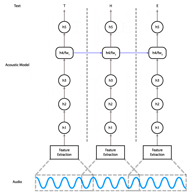
An alternative architecture that uses a unidirectional RNN in which each time step only depends on the input at that time and the state from the previous step.

Here’s code for creating an inference graph that can keep track of the state between each input window:

import tensorflow as tf

def create_inference_graph(batch_size=1, n_steps=16, n_features=26, width=64):
    input_ph = tf.placeholder(dtype=tf.float32,
                              shape=[batch_size, n_steps, n_features],
                              name='input')
    sequence_lengths = tf.placeholder(dtype=tf.int32,
                                      shape=[batch_size],
                                      name='input_lengths')
    previous_state_c = tf.get_variable(dtype=tf.float32,
                                       shape=[batch_size, width],
                                       name='previous_state_c')
    previous_state_h = tf.get_variable(dtype=tf.float32,
                                       shape=[batch_size, width],
                                       name='previous_state_h')
    previous_state = tf.contrib.rnn.LSTMStateTuple(previous_state_c, previous_state_h)

    # Transpose from batch major to time major
    input_ = tf.transpose(input_ph, [1, 0, 2])

    # Flatten time and batch dimensions for feed forward layers
    input_ = tf.reshape(input_, [batch_size*n_steps, n_features])

    # Three ReLU hidden layers
    layer1 = tf.contrib.layers.fully_connected(input_, width)
    layer2 = tf.contrib.layers.fully_connected(layer1, width)
    layer3 = tf.contrib.layers.fully_connected(layer2, width)

    # Unidirectional LSTM
    rnn_cell = tf.contrib.rnn.LSTMBlockFusedCell(width)
    rnn, new_state = rnn_cell(layer3, initial_state=previous_state)
    new_state_c, new_state_h = new_state

    # Final hidden layer
    layer5 = tf.contrib.layers.fully_connected(rnn, width)

    # Output layer
    output = tf.contrib.layers.fully_connected(layer5, ALPHABET_SIZE+1, activation_fn=None)

    # Automatically update previous state with new state
    state_update_ops = [
        tf.assign(previous_state_c, new_state_c),
        tf.assign(previous_state_h, new_state_h)
    ]
    with tf.control_dependencies(state_update_ops):
        logits = tf.identity(logits, name='logits')

    # Create state initialization operations
    zero_state = tf.zeros([batch_size, n_cell_dim], tf.float32)
    initialize_c = tf.assign(previous_state_c, zero_state)
    initialize_h = tf.assign(previous_state_h, zero_state)
    initialize_state = tf.group(initialize_c, initialize_h, name='initialize_state')

    return {
        'inputs': {
            'input': input_ph,
            'input_lengths': sequence_lengths,
        },
        'outputs': {
            'output': logits,
            'initialize_state': initialize_state,
        }
    }

The graph created by the code above has two inputs and two outputs. The inputs are the sequences and their lengths. The outputs are the logits and a special “initialize_state” node that needs to be run at the beginning of a new sequence. When freezing the graph, make sure you don’t freeze the state variables previous_state_h and previous_state_c.

Here’s code for freezing the graph:

from tensorflow.python.tools import freeze_graph

freeze_graph.freeze_graph_with_def_protos(
        input_graph_def=session.graph_def,
        input_saver_def=saver.as_saver_def(),
        input_checkpoint=checkpoint_path,
        output_node_names='logits,initialize_state',
        restore_op_name=None,
        filename_tensor_name=None,
        output_graph=output_graph_path,
        initializer_nodes='',
        variable_names_blacklist='previous_state_c,previous_state_h')

With these changes to the model, we can use the following approach on the client side:

1. Run the “initialize_state” node.
2. Accumulate audio samples until there’s enough data to feed to the model (16 time steps in our case, or 320ms).
3. Feed through the model, accumulate outputs somewhere.
4. Repeat 2 and 3 until data is over.

It wouldn’t make sense to drown readers with hundreds of lines of the client-side code here, but if you’re interested, it’s all MPL 2.0 licensed and available on GitHub. We actually have two different implementations, one in Python that we use for generating test reports, and one in C++ which is behind our official client API.

Performance improvements

What does this all mean for our STT engine? Well, here are some numbers, compared with our current stable release:

• Model size down from 468MB to 180MB
• Time to transcribe: 3s file on a laptop CPU, down from 9s to 1.5s
• Peak heap usage down from 4GB to 20MB (model is now memory-mapped)
• Total heap allocations down from 12GB to 264MB

Of particular importance to me is that we’re now faster than real time without using a GPU, which, together with streaming inference, opens up lots of new usage possibilities like live captioning of radio programs, Twitch streams, and keynote presentations; home automation; voice-based UIs; and so on. If you’re looking to integrate speech recognition in your next project, consider using our engine!

Here’s a small Python program that demonstrates how to use libSoX to record from the microphone and feed it into the engine as the audio is being recorded.

import argparse
import deepspeech as ds
import numpy as np
import shlex
import subprocess
import sys

parser = argparse.ArgumentParser(description='DeepSpeech speech-to-text from microphone')
parser.add_argument('--model', required=True,
                    help='Path to the model (protocol buffer binary file)')
parser.add_argument('--alphabet', required=True,
                    help='Path to the configuration file specifying the alphabet used by the network')
parser.add_argument('--lm', nargs='?',
                    help='Path to the language model binary file')
parser.add_argument('--trie', nargs='?',
                    help='Path to the language model trie file created with native_client/generate_trie')
args = parser.parse_args()

LM_WEIGHT = 1.50
VALID_WORD_COUNT_WEIGHT = 2.25
N_FEATURES = 26
N_CONTEXT = 9
BEAM_WIDTH = 512

print('Initializing model...')

model = ds.Model(args.model, N_FEATURES, N_CONTEXT, args.alphabet, BEAM_WIDTH)
if args.lm and args.trie:
    model.enableDecoderWithLM(args.alphabet,
                              args.lm,
                              args.trie,
                              LM_WEIGHT,
                              VALID_WORD_COUNT_WEIGHT)
sctx = model.setupStream()

subproc = subprocess.Popen(shlex.split('rec -q -V0 -e signed -L -c 1 -b 16 -r 16k -t raw - gain -2'),
                           stdout=subprocess.PIPE,
                           bufsize=0)
print('You can start speaking now. Press Control-C to stop recording.')

try:
    while True:
        data = subproc.stdout.read(512)
        model.feedAudioContent(sctx, np.frombuffer(data, np.int16))
except KeyboardInterrupt:
    print('Transcription:', model.finishStream(sctx))
    subproc.terminate()
    subproc.wait()

Finally, if you’re looking to contribute to Project DeepSpeech itself, we have plenty of opportunities. The codebase is written in Python and C++, and we would love to add iOS and Windows support, for example. Reach out to us via our IRC channel or our Discourse forum.